Spectral analysis of sleep electroencephalography
Source:vignettes/Spectral_analysis_sleep_electroencephalography.Rmd
Spectral_analysis_sleep_electroencephalography.RmdThis vignette provides a basic introduction to spectral analysis of electroencephalography (EEG) signal from a sleep record file.
EEG refers to all the methods of recording, analysis and interpretation of the electrical activity of the brain. In clinical EEG, multiple electrodes are usually placed on the scalp, measuring its superficial activity over time. Electrodes are typically arranged using the standardized International 10-20 system Niedermeyer and Lopes da Silva (2005), in order to enhance analysis reproducibility.
EEG is a major component in sleep analysis. Sleep stages, such as slow wave sleep or paradoxical sleep are partly defined over visual EEG characteristics (“AASM Scoring Manual - American Academy of Sleep Medicine,” n.d.). Many sleep related disorders can be identified in EEG data. Polysomnography (PSG), the gold standard exam in sleep medicine, includes EEG along many other physiological signals Ibáñez, Silva, and Cauli (2018).
Sleep data
Sleep records are usually stored using European Data Format (EDF) Kemp et al. (1992). The R package edfReader reads .edf files. Reading an .edf file takes two steps: First reading the headers of the file, then reading the selected signals. The following spectral analysis will be performed on a single channel of the EEG, the C3-M2 central derivation.
library(edfReader)

download.file(
  url = "https://rsleep.org/data/15012016HD.edf",
  destfile = "15012016HD.edf",
  method = 'curl')

h <- readEdfHeader("15012016HD.edf")

s <- readEdfSignals(h, signals = "C3-M2")
The rsleep function spectrogram() plots the spectrogram of the signal. But first, install rsleep latest version from Github.
devtools::install_github("boupetch/rsleep")

library(rsleep)

spectrogram(
  signal = s$signal,
  sRate = s$sRate,
  startTime = s$startTime)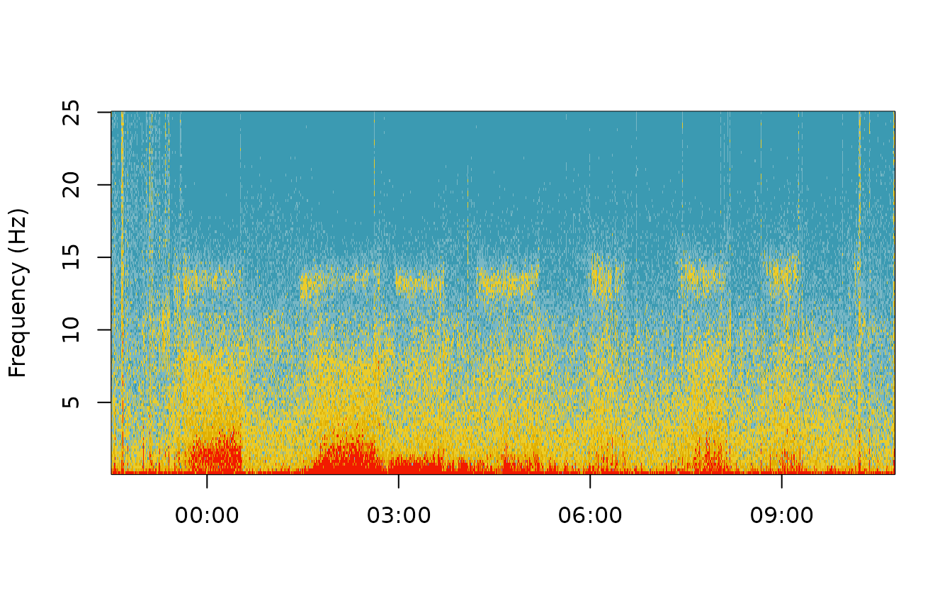
rsleep reads this particular format with the read_events_noxturnal function. The plot_hypnogram function then plots the hypnogram.
download.file(
  url = "https://rsleep.org/data/15012016HD.csv",
  destfile = "15012016HD.csv")

events <- rsleep::read_events_noxturnal("15012016HD.csv")

rsleep::plot_hypnogram(events)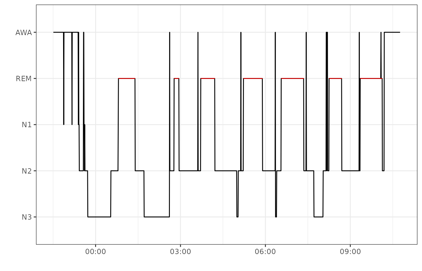
The hypnogram show sleep stages over time using consecutive 30 seconds epochs. This record was manually scored by well-trained technicians according to the American Academy of Sleep Medicine manual (“AASM Scoring Manual - American Academy of Sleep Medicine,” n.d.). Five sleep stages can be observed:
- AWA: Awakeness.
- REM: Rapid-Eye-Movement (REM) sleep, or paradoxical sleep, highlighted in red.
- N1: Light sleep transitional stage.
- N2: Light sleep.
- N3: Slow-wave sleep.
Visual scoring is an empirical science requiring a considerable amount of knowledge and training. Alternative methods like spectral estimations techniques such as the Fourier transform must be used to quantify information carried in the physiological signals Tong and Thakor (2009).
Epoching
Epoching is the first step of sleep analysis. Physiological signal, such as EEG, is splitted into consecutive epochs of a discrete duration. Epochs usually start at lights turnoff, when the patient or subject starts the night.
As the example record already has a hynogram, the EEG signal can be splitted using these scored epochs. The epochs function from the rsleep package split the signal according to these parameters. It returns a list of signal vectors.
epochs <- epochs(
  signals = s$signal,
  sRates = s$sRate,
  epoch = events,
  startTime = as.numeric(as.POSIXct(h$startTime)))
Periodogram
The Fourier transform (FT) may be the most important function in signal analysis. It decomposes the signal into its constituent frequencies and computes its power spectral densities (PSD). However, EEG signals also carry a lot of noise. This noise is easily intereprted by the FT and can jam the results. To solve this problem, Welch’s method split the signal into overlapping segments to average power spectral densities from the Fourier transform.
Single epoch
The pwelch function rsleep computes a periodogram using Welch’s method. The following example computes and plot the periodogram of the 120th epoch. This epoch has been scored N2, or light sleep, by the expert.
p <- pwelch(epochs[[120]], sRate = s$sRate)
summary(p)
#>        hz           psd
#>  Min.   :  0   Min.   :-12.007
#>  1st Qu.: 25   1st Qu.:-11.132
#>  Median : 50   Median :-10.343
#>  Mean   : 50   Mean   : -9.128
#>  3rd Qu.: 75   3rd Qu.: -7.909
#>  Max.   :100   Max.   :  0.000
This epoch periodogram shows high PSD in lower frequencies of the spectrum. As values are normalized using log, PSD are negative.
Stages profiles
To compute average periodograms by stage, hypnogram and epochs can be iterated simultaneously using the mapply function. Periodograms can be filtered at this step to discard values over 30 Hertz.
periodograms <- mapply(
  x = epochs,
  y = events$event,
  FUN = function(x,y){
    p <- pwelch(x, sRate = s$sRate, show = FALSE)
    p <- as.data.frame(p[p$hz <= 30,])
    p$stage <- y
    p
}, SIMPLIFY = F)
mapply returns a list that can be coerced to a dataframe using rbind combined to do.call.
periodograms_df <- do.call("rbind", periodograms)Once coerced to a dataframe, raw periodogram values can be averaged by stage.
avg_periodograms <- aggregate(psd ~ hz+stage, periodograms_df, mean)Aggregated periodograms can then be plotted using ggplot2.
library(ggplot2)

palette <- c("#5BBCD6","#00A08A","#F2AD00","#F98400","#FF0000")

ggplot(avg_periodograms, aes(x=hz,y=psd,color=stage)) +
  geom_line() + theme_bw() +
  theme(legend.title = element_blank()) +
  scale_colour_manual(name = "stage",
                      values = palette) +
  xlab("Frequency (Hertz)") + ylab("PSD")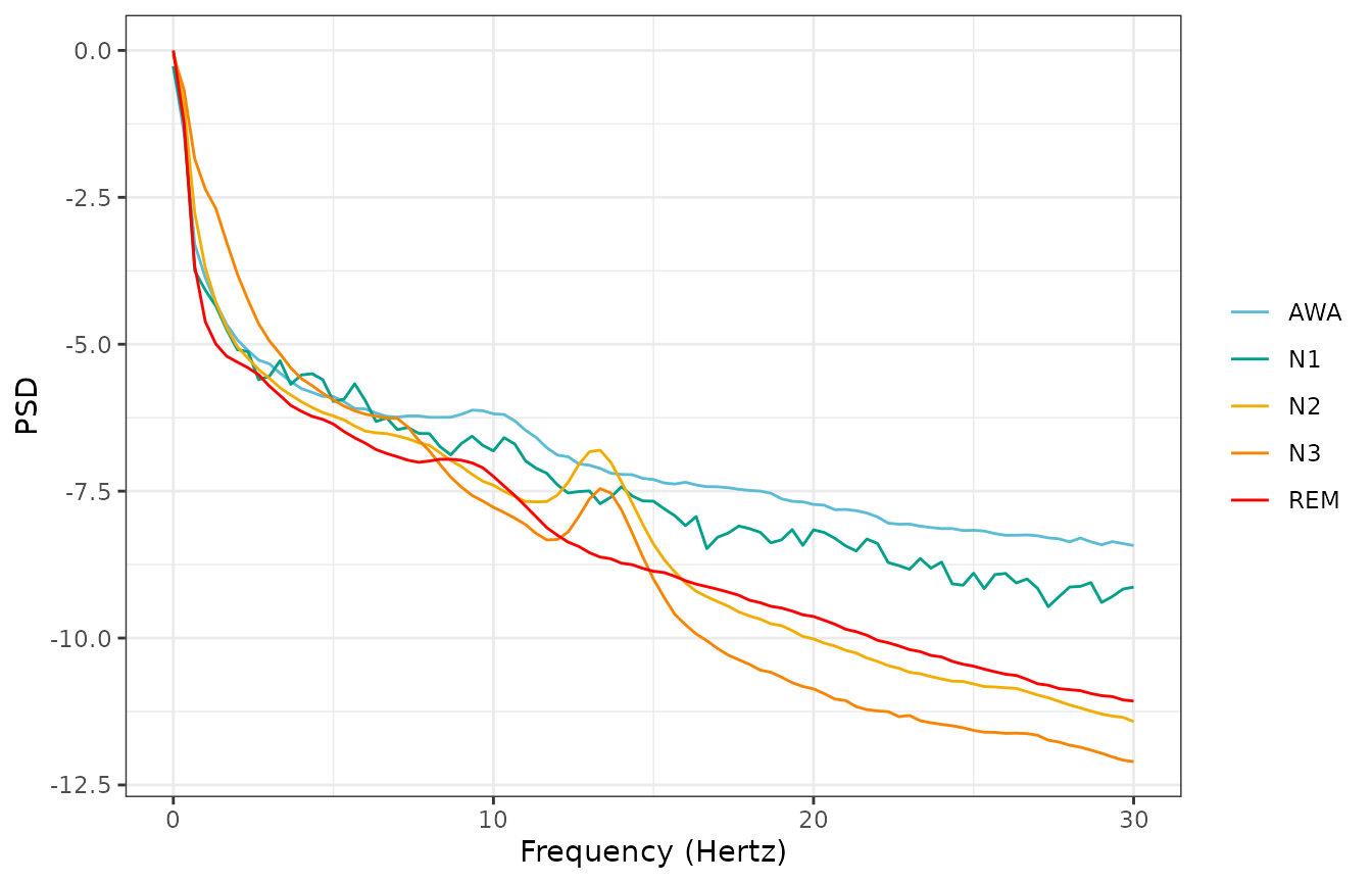
Each sleep stage show a distinct average periodogram. If the N3 stage averages higher PSD values in the lower spectrum, it show way lower PSD in the upper frequencies compared to other stages.
Bands
The traditional way to simplify the EEG periodogram is to cut the frequencies of the spectrum into bands or ranges Niedermeyer and Lopes da Silva (2005):
Delta: Below
3.5Hertz, the Delta band is associated with slow-wave sleep in adults subjects.Theta: Between
3.5and7.5Hertz, the Theta band is associated with drowsiness in adults and teens subjects.Alpha: Between
7.5and13Hertz, the Alpha band is associated with a relaxed state and eyes closed.Beta: Between
13and30Hertz the Beta band is associated with active thinking, focus, high alert or anxiousness.Gamma: Over
30Hertz the Gamma band is where are the fastest and less understood waves. They are thought to be involved in higher mental activities and integration of information.
Bands can be computed using the bands_psd of the rsleep package. Those bands can be normalized by the spectrum range covered by the bands.
bands <- lapply(epochs,function(x){
    bands_psd(
      bands = list(c(0.5,3.5), # Delta
                   c(3.5,7.5), # Theta
                   c(7.5,13), # Alpha
                   c(13,30)), # Beta
      signal = x, sRate = s$sRate, normalize = TRUE)
})
As lapply returns a list, results must be reshaped in order to obtain a dataframe object.
bands_df <- data.frame(matrix(unlist(bands), nrow=length(bands), byrow=TRUE))

colnames(bands_df) <- c("Delta","Theta","Alpha","Beta")
Stages can be retreived from the hypnogram.
bands_df$stage <- rsleep::hypnogram(events)$eventNow that the epochs bands PSD and their corresponding stages are stored in a dataframe, they can easily be plotted using boxplots from ggplot2.
bands_df_long <- reshape2::melt(bands_df, "stage")

palette <-c("#F98400", "#F2AD00", "#00A08A", "#FF0000", "#5BBCD6")

ggplot(bands_df_long,
       aes(x=stage,y=value,color=stage)) +
  geom_boxplot() +
  facet_grid(rows = vars(variable),scales = "free") +
  scale_colour_manual(name = "stage",
                      values = palette) +
  theme_bw() + xlab("") + ylab("PSD") +
  theme(legend.position = "none")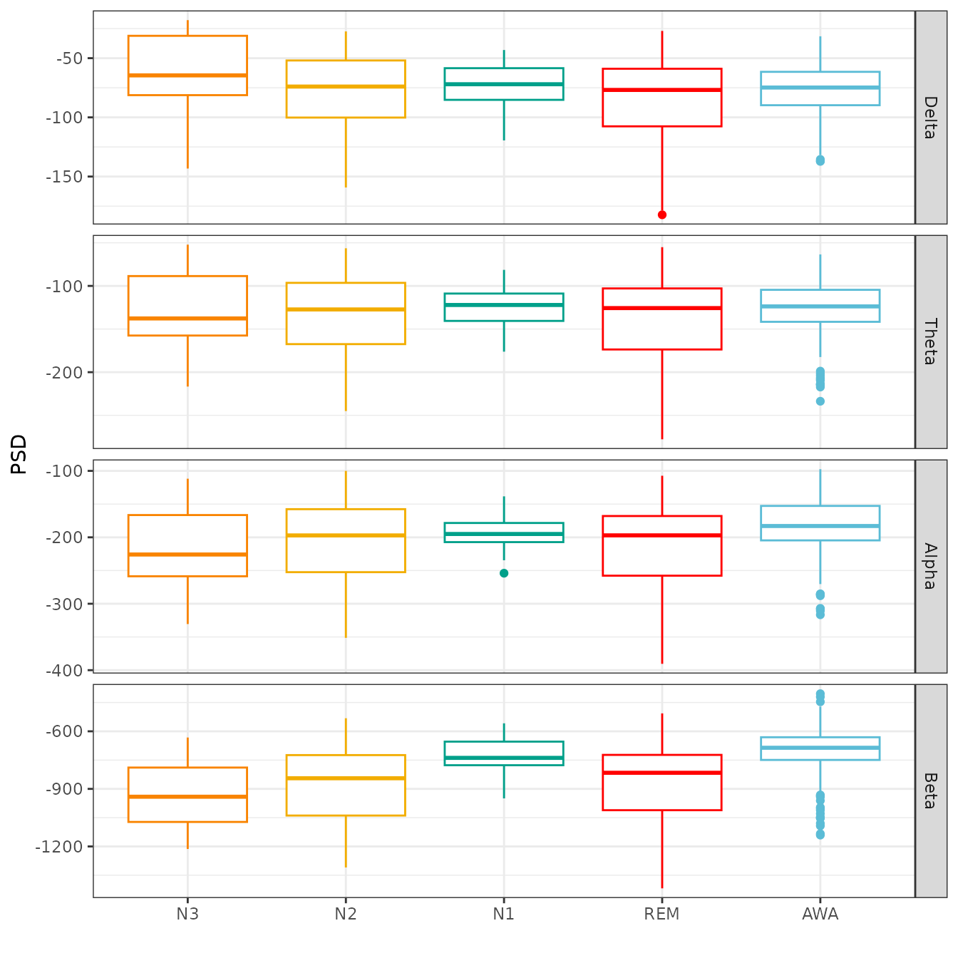
Once normalized, bands powers displayed over epoch numbers reveals the dynamic interplay of brain activity overnight.
bands_df$stage = NULL

bands_df_normalized = as.data.frame(sapply(bands_df, function(x) {
  return((x - min(x)) / (max(x) - min(x)))
}))

bands_df_normalized$epoch = c(1:nrow(bands_df_normalized))

long_bands_df_normalized <- reshape2::melt(
  bands_df_normalized, id.vars = "epoch")

ggplot(
  long_bands_df_normalized,
  aes(x = epoch, y = value, color = variable)) +
  geom_line(size = 0.4) +
  labs(title = "Bands power overnight", x = "Epoch ", y = "PSD") +
  theme_minimal() +
  scale_color_manual(values = c("#00A08A", "#F2AD00", "#F98400", "#5BBCD6")
) +
  theme(legend.position = "bottom", legend.title = element_blank())
#> Warning: Using `size` aesthetic for lines was deprecated in ggplot2 3.4.0.
#> ℹ Please use `linewidth` instead.
#> This warning is displayed once every 8 hours.
#> Call `lifecycle::last_lifecycle_warnings()` to see where this warning was
#> generated.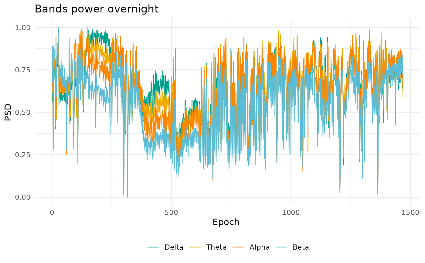
References
“AASM Scoring Manual - American Academy of Sleep Medicine.” n.d. American Academy of Sleep Medicine Association for Sleep Clinicians and Researchers. https://aasm.org/clinical-resources/scoring-manual/.
Ibáñez, Vanessa, Josep Silva, and Omar Cauli. 2018. “A Survey on Sleep Assessment Methods.” PeerJ 6 (May): e4849. https://doi.org/10.7717/peerj.4849.
Kemp, Bob, Alpo Värri, Agostinho C. Rosa, Kim D. Nielsen, and John Gade. 1992. “A simple format for exchange of digitized polygraphic recordings.” Electroencephalography and Clinical Neurophysiology 82 (5): 391–93. https://doi.org/10.1016/0013-4694(92)90009-7.
Niedermeyer, Ernst, and F. H. Lopes da Silva, eds. 2005. Electroencephalography: Basic Principles, Clinical Applications, and Related Fields. 5th ed. Philadelphia: Lippincott Williams & Wilkins.
Tong, Shanbao, and Nitish Vyomesh Thakor, eds. 2009. Quantitative EEG Analysis Methods and Clinical Applications. Artech House Series Engineering in Medicine & Biology. Boston: Artech House.