A7 spindle detection algorithm

A sleep spindle detection algorithm that emulates human expert spindle scoring

a7(
  x,
  sRate,
  window = 0.3,
  step = 0.1,
  butter_order = 5,
  A7absSigPow = 1.25,
  A7relSigPow = 1.6,
  A7sigmaCov = 1.3,
  A7sigmaCorr = 0.69
)

Arguments

x

EEG signal in uV.

sRate

Sample rate of the signal.

window

Size of the window in seconds. Default: 0.3

step

Size of the step between windows in seconds. Default: 0.1

butter_order

Order of the Butterworth filters. Default: 5

A7absSigPow

A7absSigPow treshold. Default: 1.25

A7relSigPow

A7relSigPow treshold. Default: 1.6

A7sigmaCov

A7sigmaCov treshold. Default: 1.3

A7sigmaCorr

A7sigmaCorr treshold. Default: 0.69

Value

Detected spindles and associated features.

Details

A sleep spindle detection algorithm based on 4 features computed along segmented signal according to `window` size and `step` size parameters.

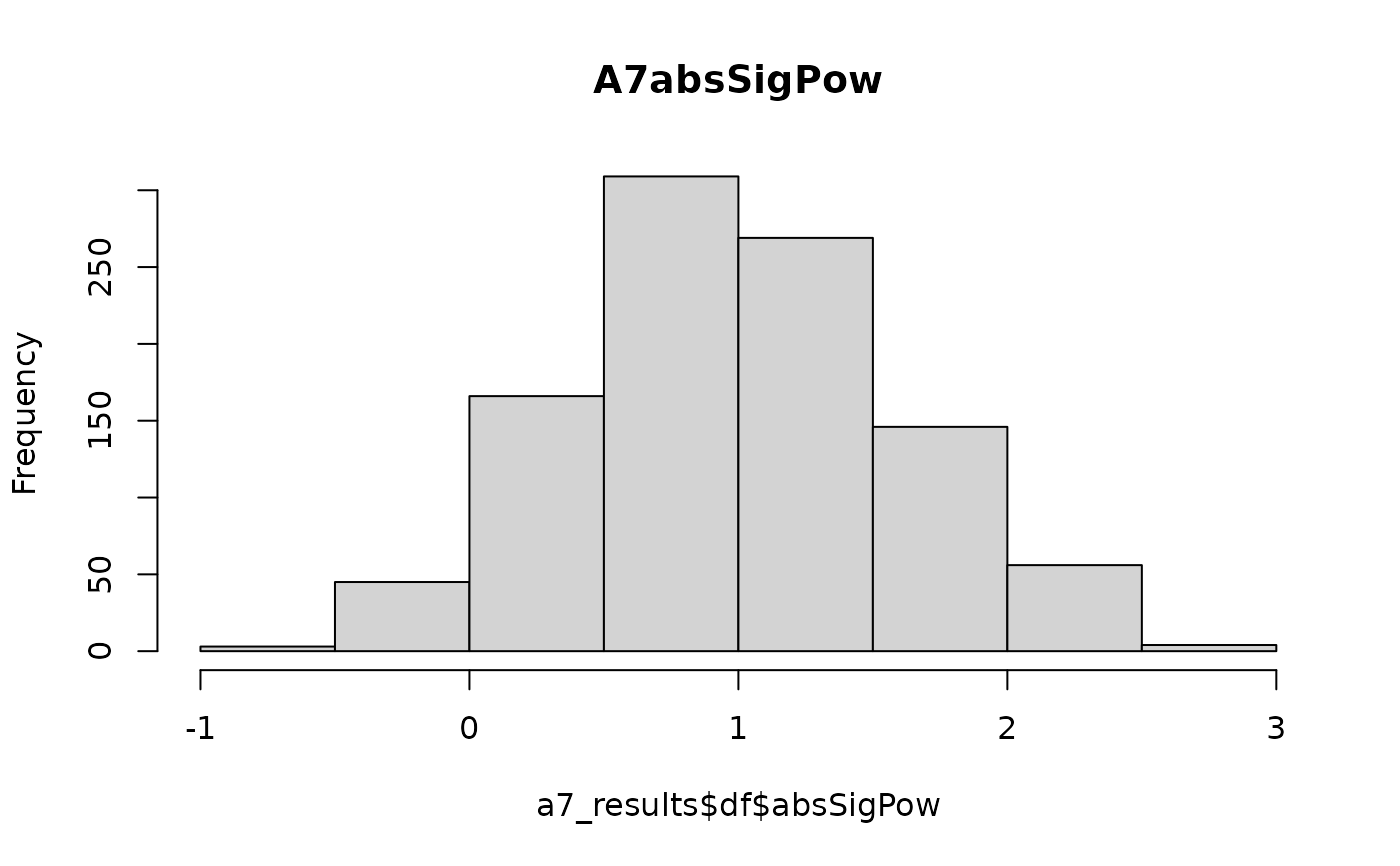
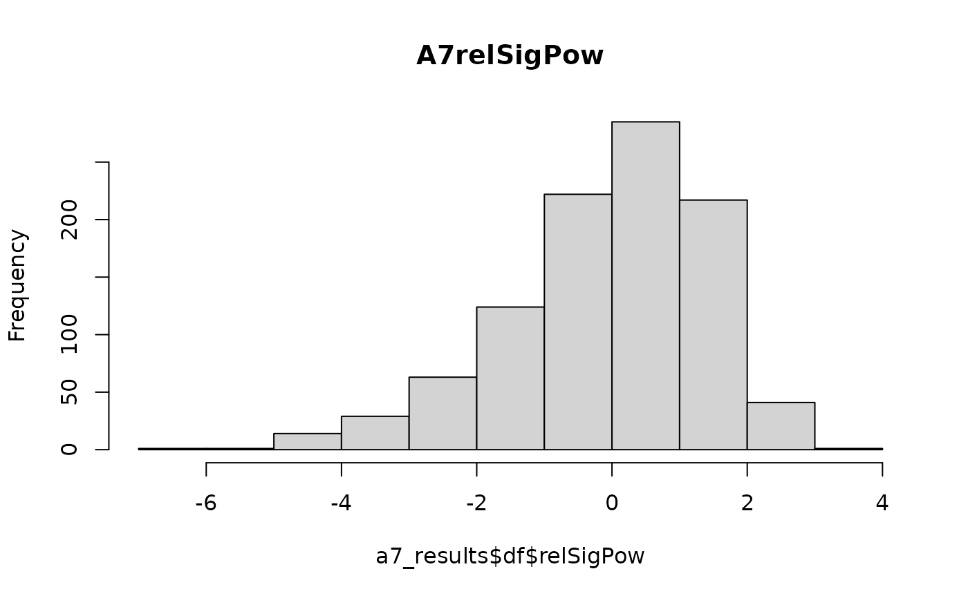
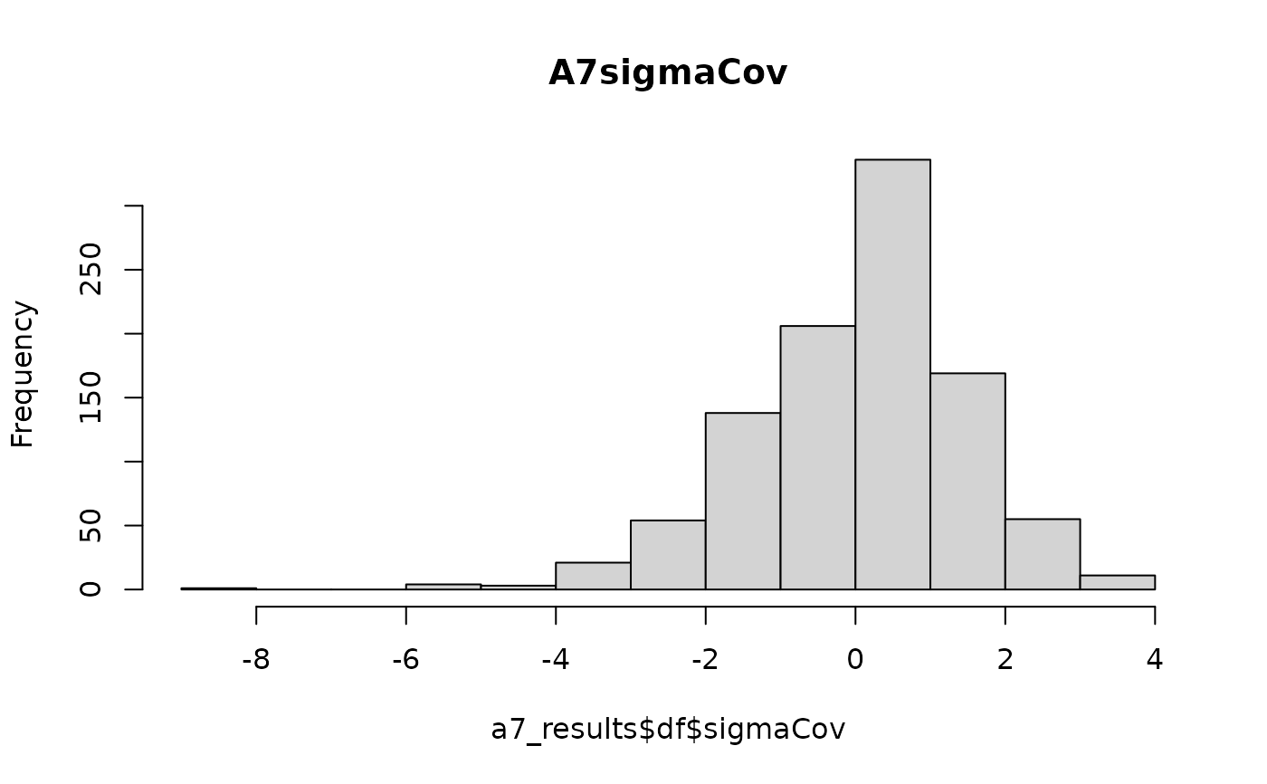
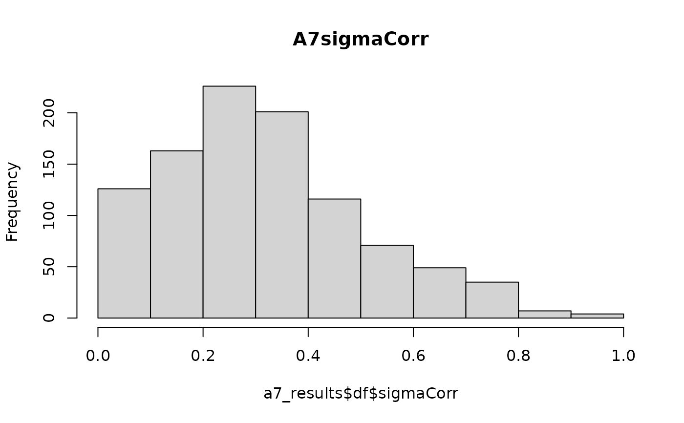
1. Absolute sigma power $$A7absSigPow = \log_{10} \left( \sum_{i=1}^{N} \frac{EEG\sigma_{i}^2}{N} \right)$$ 2. Relative sigma power $$A7relSigPow = zscore\left( \log_{10} \left( \frac{PSA_{11-16Hz}}{PSA_{4.5-30Hz}} \right) \right)$$ 3. Sigma covariance $$A7sigmaCov = zscore\left( \log_{10} \left( \frac{1}{N} \sum_{i=1}^{N} \left( EEG_{bf_i} - \mu_{EEG_{bf}} \right) \left( EEG_{\sigma_i} - \mu_{EEG_{\sigma}} \right) \right) \right)$$ 4. Sigma correlation $$A7sigmaCor = \frac{\text{cov}(EEG_{bf}, EEG_{\sigma})}{sd_{EEG_{bf}} * sd_{EEG_{\sigma}}}$$

References

Lacourse, K., Delfrate, J., Beaudry, J., Peppard, P., & Warby, S. C. (2019). A sleep spindle detection algorithm that emulates human expert spindle scoring. In Journal of Neuroscience Methods (Vol. 316, pp. 3–11). Elsevier BV. https://doi.org/10.1016/j.jneumeth.2018.08.014

Examples

tryCatch({
  fpath <- paste0(tempdir(),"c3m2_n2_200hz_uv.csv")

  download.file(
    url = "https://rsleep.org/data/c3m2_n2_200hz_uv.csv",
    destfile = fpath)

  # Read only a sample of the EEG signal
  s = read.csv(fpath,header = FALSE)[,1][25000:45000]

  file.remove(fpath)

  a7_results = a7(s, 200)

  # Plot the first detected spindle
  data = data.frame(x=s,index=seq_along(s))
  a = a7_results$spindles$idxStart[1]
  b = a7_results$spindles$idxEnd[1]
  data = data[(data$index <= (b+600)) & (data$index >= (a-600)), ]
  library(ggplot2)
  ggplot(data, aes(x = index, y = x)) +
    geom_line() +
    geom_line(data = subset(data, index >= a & index <= b), aes(x = index, y = x), color = "red") +
    labs(x = "Signal index", y = "C3-M2") +
    theme_minimal()
  
  # Visualise features distribution 

  hist(a7_results$df$absSigPow,main = "A7absSigPow")

  hist(a7_results$df$relSigPow,main = "A7relSigPow")

  hist(a7_results$df$sigmaCov,main = "A7sigmaCov")

  hist(a7_results$df$sigmaCorr,main = "A7sigmaCorr") 
 }, error = function(e) {
  print("Error executing this example, check your internet connection.")
  })